The word ‘demand’ is so common and familiar with every one of us that it seems superfluous to define it. The need for a precise definition arises simply because it is sometimes confused with other words such as desire, wish, want, etc.
Demand in economics means a desire to possess a good supported by the willingness and ability to pay for it. If you have a desire to buy a certain commodity, say a car, but you do not have the adequate means to pay for it, it will simply be a wish, a desire, or a want and not demand.
Demand is an effective desire, i.e., a desire that is backed by willingness and ability to pay for a commodity in order to obtain it. In the words of Prof. Hibdon:
“Demand means the various quantities of goods that would be purchased per time period at different prices in a given market.”
Characteristics of Demand:
There are three main characteristics of demand in economics.
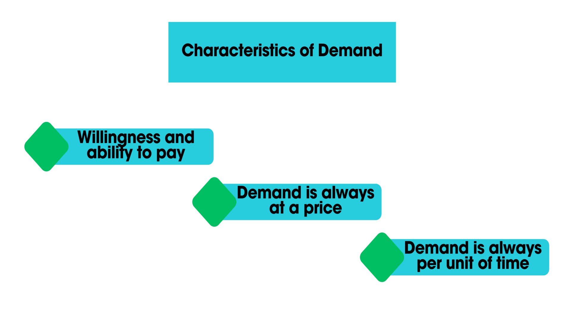
Willingness and ability to pay
Demand is the amount of a commodity for which a consumer has the willingness and also the ability to buy.
Demand is always at a price
If we talk of demand without reference to price, it will be meaningless. The consumer must know both the price and the commodity. He will then be able to tell the quantity demanded by him.
Demand is always per unit of time
The time may be a day, a week, a month, or a year.
Example: For instance, when milk is selling at the rate of $60 per liter, the demand of a buyer for milk is 10 liters a day. If we do not mention the period of time, nobody can guess as to how much milk we consume. It is just possible we may be consuming ten liters of milk a week, a month, or a year.
Summing up, we can say that by demand is meant the amount of the commodity that buyers are able and willing to purchase at any given price over some given period of time.
Demand is also described as a schedule of how much a good people will purchase at any price during a specified period of time.
Law of Demand:
Definition and Explanation of the Law:
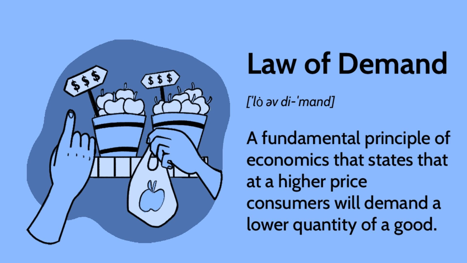
We have stated earlier that demand for a commodity is related to the price per unit of time. It is the experience of every consumer that when the prices of commodities fall, they are tempted to purchase more commodities, and when the prices rise, the quantity demanded decreases.
There is, thus, an inverse relationship between the price of the product and the quantity demanded. Economists have named this inverse relationship between demand and price as the law of demand.
Statement of the Law:
Some well-known statements of the law of demand are as under:
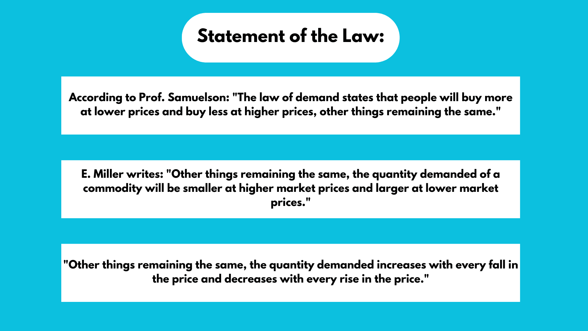
- According to Prof. Samuelson: “The law of demand states that people will buy more at lower prices and buy less at higher prices, other things remaining the same.”
- E. Miller writes: “Other things remaining the same, the quantity demanded of a commodity will be smaller at higher market prices and larger at lower market prices.”
- “Other things remaining the same, the quantity demanded increases with every fall in the price and decreases with every rise in the price.”
In simple terms, we can say that when the price of a commodity rises, people buy less of that commodity, and when the price falls, people buy more of it ceteris paribus (other things remaining the same). Or we can say that the quantity varies inversely with its price.
There is no doubt that demand responds to price in the reverse direction, but it has got no uniform relation between them. If the price of a commodity falls by 1%, it is not necessary that demands may also increase by 1%. The demand can increase by 1%, 2%, 10%, 15%, as the situation demands.
The functional relationship between demand and the price of the commodity can be expressed in simple mathematical language as under:
Formula for Law of Demand:

Qdx = f(Px, M, P°, T, ……)
Here,
Qd^x = A quantity demanded of commodity x.
f = A function of independent variables contained within the parenthesis.
P^x = Price of commodity x.
P° = Price of other commodities.
T = Taste of the household.
M = Purchasing power of the typical consumer.
If M, P°, and T are kept constant, then the demand function can also be symbolized as:
Qd^x = f(P^x) ceteris paribus.
Ceteris Paribus: In economics, the term is used as shorthand for indicating the effect of one economic variable on another, holding constant all other variables that may affect the second variable.
Schedule of Law of Demand
The demand schedule of an individual for a commodity is a list or table of the different amounts of the commodity that are purchased in the market at different prices per unit of time. An individual demand schedule for a good, say a shirt, is presented in the table below:
Demand Schedule for Shirts:
| Price per shirt (Px) | 100 | 78 | 60 | 40 | 20 | 10 |
| Quantity demanded per year (Qdx) | 5 | 7 | 9 | 13 | 20 | 30 |
According to this demand schedule, an individual buys 5 shirts at $100 per shirt and 30 shirts at $10 per shirt in a year.
Law of Demand Curve/Diagram
Demand curve is a graphical representation of the demand schedule. According to Lipsey, “This curve, which shows the relation between the price of a commodity and the amount of that commodity the consumer wishes to purchase is called demand curve”.
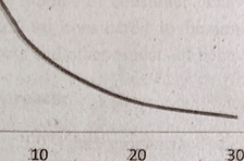
In Figure 3.1, the quantity demanded of shirts is plotted on the horizontal axis, and price is measured on the vertical axis. Each price-quantity combination is plotted as a point on this graph.
If we join the price-quantity points, we get the individual demand curve for shirts. The demand curve slopes downward from left to right.
It has a negative slope, showing that the two variables, such as price and quantity, work in opposite directions.
When the price of a good rises, the quantity demanded decreases, and when its price decreases, quantity demanded increases, ceteris paribus.
Assumptions of the Law of Demand
According to Prof. Stigler and Boulding, there are three main assumptions of the Law:
- There should not be any change in the tastes of the consumers for goods (T).
- The purchasing power of the typical consumer must remain constant (M).
- The price of all other commodities should not vary (P°).
Limitations/Exceptions of the Law of Demand

Though, as a rule, when the prices of normal goods rise, then the demand decreases, but there may be a few cases where the law may not operate.
- Prestigious goods: There are certain commodities like diamond, sports cars, etc., which are purchased as a mark of distinction in society. If the price of these goods rises, the demand for them may increase instead of falling.
- Price expectations: If people expect a further rise in the price of a particular commodity, they may buy more in spite of the rise in price. The violation of the law in this case is only temporary.
- Ignorance of the consumer: If the consumer is ignorant about the rise in the price of goods, he may buy more at a higher price.
- Giffen goods: If the price of basic goods (potatoes, sugar, etc.) falls, then the demand for those goods also falls because with the surplus income through falling prices, people buy superior goods.
Slope of the Demand Curve
The demand curve generally slopes downward from left to right. It has a negative slope because the two important variables, price and quantity, work in opposite directions.
As the price of a commodity decreases, the quantity demanded increases over a specified period of time, and vice versa, other things remaining constant. The fundamental reasons for the demand curve to slope downward are as follows:
Law of diminishing marginal utility
The law of demand is based on the law of diminishing marginal utility. According to the cardinal utility approach, its marginal utility declines when a consumer purchases more commodity units. The consumer, therefore, will purchase more units of that commodity only if its price falls.
Thus, a price decrease brings about an increase in demand. The demand curve, therefore, is downward sloping.
Income effect
Other things being equal, when a commodity’s price decreases, the household’s real income or purchasing power increases.
The consumer is now able to purchase more commodities with the same income. The demand for a commodity thus increases not only from existing buyers but also from new buyers who were earlier unable to purchase at a higher price.
When, at a lower price, there is a greater demand for a commodity by households, the demand curve is bound to slope downward from left to right.
Substitution effect
The demand curve slopes downward from left to right also because of the substitution effect. For instance, the price of meat falls, and the prices of other substitutes, say poultry and beef, remain constant.
Then the households would prefer to purchase meat because it is now relatively cheaper. The increase in demand with a fall in the price of meat will move the demand curve downward from left to right.
Entry of new buyers
When the price of a commodity falls, its demand increases not only from the old buyers but also from new buyers who enter the market. The combined result of the income and substitution effect is that demand extends, ceteris paribus, as the price falls. The demand curve slopes downward from left to right.
Importance of the Law of Demand

Determination of price
The study of the law of demand is helpful for a trader to fix the price of a commodity. He knows how much demand will fall by an increase in price to a particular level and how much it will rise by a decrease in the price of the commodity.
The schedule of market demand can provide information about the total market demand at different prices. It helps the management in deciding how much increase or decrease in the price of the commodity is desirable.
Importance to Finance Minister
The study of this law is of great advantage to the finance minister. If by raising the tax the price increases to such an extent that the demand is reduced considerably, then it is of no use to raise the tax because revenue will almost remain the same.
The tax will be levied at a higher rate only on those goods whose demand is not likely to fall substantially with the increase in price.
Importance to the Farmers
Good or bad crop affects the economic condition of the farmers. If a good crop fails to increase the demand, the price of the crop will fall heavily. The farmer will have no advantage of the good crop, and vice-versa.
Summing up, we can say that the limitations or exceptions of the law of demand stated above do not falsify the general law. It must operate.
Individual’s Demand for a Commodity
“The individual’s demand for a commodity is the amount of a commodity that the consumer is willing to purchase at any given price over a specified period of time”.
The individual’s demand for a commodity varies inversely with price (Ceteris paribus). As the price of a good rises, other things remaining the same, the quantity demanded decreases, and as the price falls, the quantity demanded increases.
Here, the price (p) is an independent variable, and quantity (q) is the dependent variable.
Individual’s Demand Schedule
The demand schedule of an individual for a commodity is a list or table of the different amounts of the commodity that are purchased in the market at different prices per unit of time. An individual demand schedule for a good, say shirts, is presented in the table below:
Individual Demand Schedule for Shirts:
| Price Per Shirt (Tk.) | 100 | 80 | 58 | 34 | 20 | 10 |
| Quantity Demanded Per Year, Qdx | 5 | 7 | 10 | 15 | 21 | 30 |
According to this demand schedule, an individual buys 5 shirts at $100 per shirt and 30 shirts at $10 per shirt in a year.
Individual’s Demand Curve:
Demand curve is a graphical representation of the demand schedule. According to Lipsey, “The curve, which shows the relation between the price of a commodity and the amount of that commodity the consumer wishes to purchase is called demand curve”.
It is a graphical representation of the demand schedule.
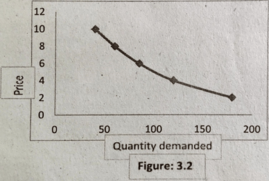
In the figure 3.2 the quantity demanded of shirts is plotted on horizontal axis and price is measured on vertical axis. Each price quantity combination is plotted as a point on this graph. If we join the price quantity points we get the individual demand curve for shirts.
The demand curve slopes downward from left to right. It has a negative slope showing that the two variables price and quantity work in opposite direction. When the price of a good rises, the quantity demanded decreases and when its price decreases, quantity .demanded increases, ceteris paribus.