Simple Random Sampling

Simple random sampling is a procedure that gives each sampling unit in the population an equal and known non-zero probability of being selected. Selecting a simple random sample may be accomplished with the aid of computer software, a table of random numbers, or a scientific calculator.

In most instances, random numbers are employed to select samples. Such a selection procedure ensures that every population unit has an equal probability of being included in the sample.

Drawing a simple random sample from a population requires that each eligible population unit be assigned an equal probability of selection in every draw. This ensures randomness in the selection making the sample independent of human judgment.

In reality, a simple random sample is drawn unit by unit.

If a list (sampling frame) of the population units is available, random sample selection may be easily accomplished using random numbers.

The following 8-step procedure may be followed in drawing a simple random sample of n units using random numbers from a population of N units.

1. Assign serial numbers to the units in the population from 1 through
2. Decide on the random number table to be used.
3. Choose an N-digit random number from any point in the random number table.
4. If this random number is less than or equal to N, this is your first selected unit.
5. Move on to the next random number not exceeding N, vertically, horizontally, or in any other direction systematically and choose your second unit.
6. If at any stage of your selection, the random number chosen exceeds N, discard it, and choose the next random number.
7. If further, any random number is repeated, it must also be discarded and be replaced by a fresh random number appearing next.
8. The process stops once you arrive at your desired sample size.

The following examples are designed to illustrate how the selection of population elements can be made in practice.

Example #1: Draw a simple random sample of size 5 from a population comprising 150 units employing a simple random sampling method.

Here n=5 and 7V=150. Assign serial numbers 001, 002,….,150 to the 150 units in the population. Since 150 is a three-digit number, we merely read three-digit random numbers presented in the Appendix.

Suppose we start from the leftmost digit of the first row of the random number table in Appendix 1 and proceed downward until we achieve a sample of 5 units.

The random numbers were as follows:

277	130	802	108	541	603	497	786	666	440
414	945	416	502	413	258	061	608	809	195
493	063	609	923	779	381	396	840	474	433
642	668	724	210	953	407	582	895	154	121

Note that we choose only those numbers, which lie in the range 001-150. Any number lying outside this range is omitted since they do not correspond to any unit in the population. The process stops once we arrive at five numbers.

Note that the selected numbers are 130, 108, 61, 63, and 121. These numbers are underlined with bold faces. All these numbers are distinct.

If a random number occurs twice, the second occurrence is omitted, and another number is selected as its replacement.

Example #2: Assume that there are 77=1000 records of daily wages of the employees of the pharmaceutical industry. Draw a sample of 25 records using the random numbers shown in Appendix 1 to draw a sample of 25 records.

The first step is to arrange the wages of 1000 employees, assigning a number from 000 to 999. That is, we have 1000 three-digit numbers where 001 represents the first record, 999 the 999^th record and 000 the 1000^th.

We may use the first three digits of the second column of random numbers in Appendix 1, consisting of 10 random digits dropping the last 7 digits of each random number. We see that the first selected number is 853, the second is 540, and the third is 985, and so on. Proceeding further down the column, the following random numbers are chosen:

853	540	985	903	266
373	920	164	998	073
495	496	641	417	906
906	715	883	744	104
467	236	159	118	782

Note that renumbering the serials has made the task of choosing the cases much easier, and there has been no rejection in the process.

If the wage records of the employees are actually numbered, we merely choose the records with the corresponding numbers, and these records represent a simple random sample of size w=25 from .¥=1000.

We illustrate below by an example a relatively efficient method of drawing a simple random sample that has less rejection rate.

Example #3: Refer to Example #1. The population from which a sample of 5 has to be chosen contains 150 units. For selecting a unit from 001- 150, follow the steps below:

1. Choose a random number from the random number table provided to you (refer to the random numbers shown in Example 5.3). This number is 277, which exceeds 150.
2. Divide 277 by 150. The remainder is 127. The unit labeled 127 in the population is your first selected unit.
3. To select the second unit, choose the next random number. This number is 130, which is less than 150. We directly choose this number as our second unit in the sample.
4. The next random number is 802, which results in a remainder of 52 when divided by 150. The unit corresponding to this number is our third selected unit.
5. Continuing this process, we arrive at the next two numbers. These are 108 and 91.
6. The random numbers thus chosen are 52, 91, 108, 127, and 130.

The procedure above is referred to as the remainder method. This procedure has the advantage of having less rejection rate in the selection process.

Determination of Sample Size in a Simple Random Sample

One of the most important problems in planning a sample survey is that of determining how large a sample is needed for the estimates to be reliable enough to meet the objectives of the survey.

The decision is important for several reasons. Too large a sample involves huge cost, manpower, materials, and time, while too small a sample invalidates the results. Then the question is: what is the optimum size of the sample?

Although general rules are hard to make for the sample size without knowledge of the specific population, around 30 cases seem to be the bare minimum for studies in which statistical data analysis is to be done (Champion 1970: 89).

However, many researchers regard 50, and some argue for 100 cases as the minimum (Fisher et al. 1991).

One reason is that there are often several sub-populations the researchers wish to study separately or several variables to be controlled for.

If there are not enough cases in each sub-group of the population, it is sometimes hard to meet the assumption of standard statistical tests such as chi-square in particular. In addition, percentages calculated on the basis of fewer than 30 cases tend to be unreliable.

Fisher et al. (1991) suggest a simple approach in the cases when one intends to analyze data in a contingency table. This approach ensures a minimum number of cases as cell frequencies in a cross-table of variables.

Following the approach, let us consider the problem of analyzing the association between mothers’ nutritional knowledge and their education level. In order to analyze such a table, two points are to be kept in mind while determining the sample size:

• Each category of the independent variable should contain at least a specified number of cases;
• Each cell’s expected number of cases should be at least 5 (to permit statistical tests, such as chi-square).

In the present example, education is the independent variable, while nutritional knowledge is the dependent variable. Let the variable ‘education’ have 4 levels as below:

Education level	% of mothers
None	60
Primary	20
Secondary	15
Above secondary	5
Total	100

Our assumption is that the above four categories constitute respectively 60%, 20%, 15%, and 5% of all respondents in the population (see column 2 in the above table).

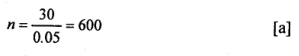
Hence in order to have a sample large enough to ensure at least 30 cases (say) in the smallest category of the variable (here 5% cases) of the total number of cases, the sample size required is

Now suppose that nutritional knowledge of the mothers has 3 categories: ‘no knowledge,’ ‘moderate knowledge’ and ‘high knowledge’ which account respectively for 30%, 20% and 50% of all mothers

Knowledge level	% of mothers
No knowledge	30
Moderate knowledge	20
High knowledge	50
Total	100

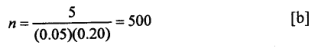
To find minimum sample size needed to ensure an expected cell frequency of at least 5, we divide 5 by the product of the proportion falling in the smallest categories of the two variables (viz.: 5% for above secondary, and 20% for moderate knowledge):

Since the sample size required must meet both criteria (30 cases in each variable category and 5 cases in each cell), the larger of the two estimates (600 vs. 500) should be adopted as the final sample size.

This criterion leads to a choice of n=600 as our final sample size. We can verify that the above procedure ensures that none of the cells contains less than 5 cases, and at the same time, the independent variable category contains at least 30 cases:

Table: Cross-table of Education and Nutritional Level
Education level
Nutrition level	None	Primary	Secondary	Above secondary	Total (%)
No knowledge	108	36	27	9	180 (30%)
Moderate knowledge	72	24	18	6	120 (20%)
High knowledge	180	60	45	15	300 (50%)
Total	360	120	90	30	600
(%)	(60%)	(20%)	(15%)	(5%)	(100%)

The cell values in the above table are calculated as the product of row and column percentages and the estimated sample size (n=600). For example, the first value of 108 is calculated as follows:

108=0.30×0.60×600

Similarly, the second value 60 in the third row is calculated as

60=0.50 x 0.20 x 600

We now present below a more statistically sound approach to determining sample size. In doing so, we consider two cases:

1. Determination of sample size (n) in estimating population proportion;
2. Determination of sample size (n) in estimating the population mean.

Sample size when estimating a population proportion

In sample surveys, we are frequently encountered with the problem of estimating population proportions or percentages such as the proportion of persons smoking, the proportion of children suffering from malnutrition, proportion of voters favoring a particular candidate, percentage of customers arriving at a superstore with a credit card and the like.

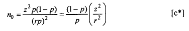
Thus if p is such a proportion that has a given attribute, then for a sufficiently large population, the formula for estimating the sample size is where:

• n₀ =desired sample size
• z =standard normal deviate usually set at 1.96, which corresponds to the 95% confidence level.
• p=assumed proportion in the target population estimated to have a particular characteristic.
• d =allowable marginal error in estimating a population proportion.

Example: A nutrition survey is to be conducted in a refugee camp. Assume that 40% of children suffer from malnutrition. How large is a sample needed in order to be 95% certain that the estimated prevalence does not differ from the true prevalence by more than 0.05?

Assuming that the population is large, we employ formula (c) above. Here z=1.96,6/=0.05 and /y=0.40. We now want to estimate the true proportion in the population within 5 percentage points of p. That is within p= 0.40 ± 0.05. Thus

If p is not known or difficult to assume, it will be the safest procedure to take it as 0.50, which maximizes the expected variance and therefore indicates a sample size that is sure to be large enough. If the proportion is expected between two values, the value closest to 50% is selected. For example, if p is thought to be between 15% and 30%, then 30%, (the larger of the two) should be chosen as the value of p to calculate n.

A common choice of d is 0.05. This value does not seem to be realistic for scenarios where the true value of p is outside the range 0.2<p<0.8 when a small value for or consideration of a relative margin of error r is recommended. The quantity r is computed as portion of the assumed true proportion p. Consideration of this relative rate of allowable error margin would convert the equation to:

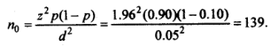
We check below that the formula (c) yields a value of 139 for n when cZ=0.5 andp=0.90:

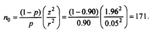
With the same values r (0.05) and p (0.90), (c*) yields:

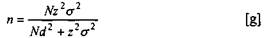
If N is small, the formula to be used assumes the following form:

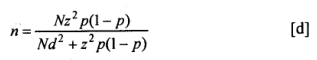
The formula (d) above can also be expressed as follows:

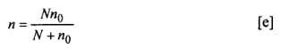
In practice, we first calculate n₀. Fi n₀/N  is negligible, then n_0o is a satisfactory approximation to n.

Assuming that p is difficult to fix in advance, we take it to be 0.50. In that event

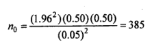
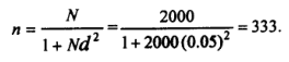
Suppose jV=2000, and we regard this as a small population. Then we would revise our estimate of n as follows:

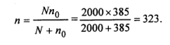
Yamane (1967) provides a more simplified formula to calculate n. This is

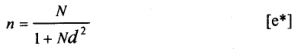
When (e*) is applied to the above case;

As can be noted, the sample size using formula (e) results in sampling of fewer children than formula (c).

It is further easy to verify that formula (c), for a given z and d values, will give the same sample size regardless of the size of the population. The following table compares the two formula numerically:

Table: Comparison of Two Sample Size Formulae for p=0.5, <£=0.05 and z=1.96
Population size	Estimated sample size when N is large	Estimated sample size when N is small
50	385	45
100	385	80
500	385	218
1,000	385	279
5,000	385	357
10,000	385	371
50,000	385	382

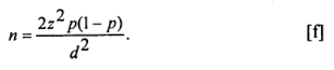
In comparative studies, one usually wants to demonstrate that there is a significant difference between the two groups. If we assume an equal number of cases (n ₁ = n ₂ = n) in the two subpopulations, the formula for n is very similar to the one above:

The sample size for estimating the population mean

Very often, we want to draw inference on the mean and the total value of variables like income, expenditure, age, or BMI.

The sample size needed to make such inference is somewhat different from the one discussed for the proportion. For the mean, the formula is where <r2 is the population variance.

Example: For a population of 10,000 women, the distribution of the body mass index (BMI) showed a variance of 15. How large a sample should we draw if we want to be 95% confident that our estimate of the average BMI in the population is off by ± 0.3?

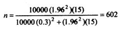
Here 7V= 10,000, a² =15, <£=0.3. Hence for estimating the mean, the sample size is obtained from (g) as below: 

Thus a sample of 602 women will be needed to achieve the desired degree of confidence in the estimate. If N were large, n would have been by virtue of (h);